In the previous post we saw how to scrape raw data from a content rich webpage. In this post, we will explore how to process that raw data and use Machine Learning tools to predict the playing role of a cricket player just based on his career statistics.
Here are the tools that we will use for this exercise. For interactive data analysis and number crunching:
- Jupyter
- Pandas
- Numpy
For visualizing data:
- Seaborn
- matplotlib
For running Machine Learning models:
- Tensorflow
- Keras
- Scikit-learn
Importing data
First let us load the necessary modules:
import matplotlib.pyplot as plt
import pandas as pd
import numpy as np
import seaborn as sns
Import the CSV file which we scraped as a pandas data frame and inspect its contents.
data = pd.read_csv('data/players.csv')
data.dtypes
—–|—- Bat_100|object Bat_4s|object Bat_50|object Bat_6s|object Bat_Ave|object Bat_BF|object Bat_Ct|int64 Bat_HS|object Bat_Inns|object Bat_Mat|int64 Bat_NO|object Bat_Runs|object Bat_SR|object Bat_St|int64 Bio_Also_known_as|object Bio_Batting_style|object Bio_Born|object Bio_Bowling_style|object Bio_Current_age|object Bio_Died|object Bio_Education|object Bio_Fielding_position|object Bio_Full_name|object Bio_Height|object Bio_In_a_nutshell|object Bio_Major_teams|object Bio_Nickname|object Bio_Other|object Bio_Playing_role|object Bio_Relation|object Bowl_10|object Bowl_4w|object Bowl_5w|object Bowl_Ave|object Bowl_BBI|object Bowl_BBM|object Bowl_Balls|object Bowl_Econ|object Bowl_Inns|object Bowl_Mat|int64 Bowl_Runs|object Bowl_SR|object Bowl_Wkts|object dtype: object|
We can see that most of the fields are decoded as object data type which is a generic pandas datatype. It gets assigned if our data consists of mixed types such as characters and numerals. There are some obvious numerical fields which are getting detected as string. But before we recast all of them as string, we need to preprocess some of them to extract numeric value out of them.
For example, let us inspect Bowl_BBI and Bowl_BBM which stands for best bowling figures in an innings and a match respectively.
data[['Bowl_BBI','Bowl_BBM']].head(n=10)
| Bowl_BBI | Bowl_BBM |
|---|---|
| 0 | - |
| 1 | 3/31 |
| 2 | 2/35 |
| 3 | - |
| 4 | - |
| 5 | - |
| 6 | - |
| 7 | - |
| 8 | 6/85 |
| 9 | - |
Either fields can be made sense as a combination of two independent variables- Best Bowling Wickets & Best Bowling Runs. Similarly when we cast the field Bat_HS as integer, the notout values will be lost since they are suffixed with an asterisk which makes them a string data type. Let us go ahead to fix these potential issues.
# Best bowling innings wickets
bbi_df = pd.DataFrame(data['Bowl_BBI'].str.replace('-','').str.split('/').tolist(),
                      columns = ['Bowl_BBIW','Bowl_BBIR'])
bbm_df = pd.DataFrame(data['Bowl_BBM'].str.replace('-','').str.split('/').tolist(),
                      columns = ['Bowl_BBMW','Bowl_BBMR'])

data = data.join([bbi_df,bbm_df])

# Identify numeric columns
numeric_cols = ['Bat_100','Bat_4s','Bat_50','Bat_6s','Bat_Ave','Bat_BF',
                'Bat_Ct','Bat_HS','Bat_Inns','Bat_Mat','Bat_NO','Bat_Runs',
                'Bat_SR','Bat_St','Bowl_10','Bowl_4w','Bowl_5w','Bowl_Ave',
                'Bowl_Balls','Bowl_Econ','Bowl_Inns','Bowl_Mat','Bowl_Runs',
                'Bowl_SR', 'Bowl_Wkts','Bowl_BBIW','Bowl_BBIR','Bowl_BBMW','Bowl_BBMR']

# regex replace * in High scores
data['Bat_HS'] = data['Bat_HS'].replace(r'\*$','',regex=True)
data[numeric_cols] = data[numeric_cols].replace('-',0)
data[numeric_cols] = data[numeric_cols].apply(pd.to_numeric, errors='coerce')
data[numeric_cols] = data[numeric_cols].fillna(0)
If we check the data type again, we will see that all the numerical fields are interpreted as int or float datatype as expected.
Be careful when filling NaN with zeroes. Idea is not to introduce false values in to the dataset. In this case, a value of zero is neutral since it represents the same value as absent numbers. But for certain types of data, such as temperature, zero introduces a false value in to the data set since temperature values can be less than zero.
Pre-processing
Deriving new features
When using data in our models we have to understand the units in which they are represented. Not all features are directly comparable. For instance, Average & Strike rates are already averaged over the number of matches that a player plays. But other aggregate statistics aren’t. So in effect it would be meaningless to compare run tally of a player who has played only 10 matches with that of another who has played a hundred matches.
To understand better, let us plot runs scored vs the matches played.
sns.jointplot(x="Bat_Runs", y="Bat_Inns", data=data)
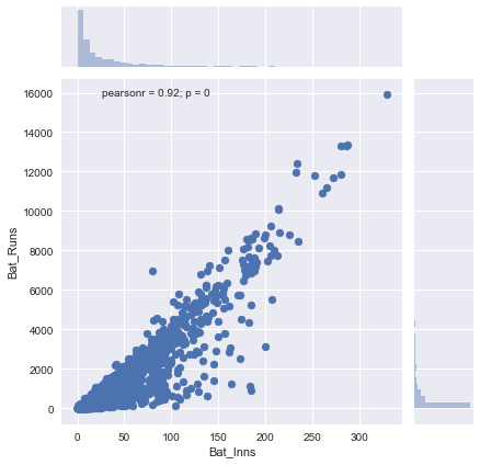
Obviously there is a strong correlation between no. of matches played and no. of runs scored. Ideally we want our features to be as independent of each other as possible. To separate the influence of number of matches played on the batting runs feature, we will divide the aggregate statistics by number of matches played.
# select aggregate stats such as no. of hundreds, runs scored etc.,
bat_features_raw = ['Bat_100', 'Bat_4s', 'Bat_50', 'Bat_6s',
                    'Bat_BF', 'Bat_Ct', 'Bat_NO', 'Bat_Runs','Bat_St']

# column names for scaled features
bat_features_scaled = ['Bat_100_sc', 'Bat_4s_sc', 'Bat_50_sc', 'Bat_6s_sc',
                    'Bat_BF_sc', 'Bat_Ct_sc', 'Bat_NO_sc', 'Bat_Runs_sc','Bat_St_sc']

# leave aside match and innings count and other aggregate stats such as best bowling figures, strike rate and average
bowl_features_raw = ['Bowl_10', 'Bowl_4w', 'Bowl_5w',
                     'Bowl_Balls', 'Bowl_Runs','Bowl_Wkts']

# column names for scaled features
bowl_features_scaled = ['Bowl_10_sc', 'Bowl_4w_sc', 'Bowl_5w_sc',
                     'Bowl_Balls_sc', 'Bowl_Runs_sc','Bowl_Wkts_sc']

# divide by innings count since it is more relevant than match count
data[bat_features_scaled] = data[bat_features_raw].apply(lambda x: x/data['Bat_Inns'])
data[bowl_features_scaled] = data[bowl_features_raw].apply(lambda x: x/data['Bowl_Inns'])

# these are the meaningful features which will be the input for our model.
features = ['Bat_Ave','Bat_HS', 'Bat_SR'] + bat_features_scaled + ['Bowl_Ave','Bowl_Econ','Bowl_SR','Bowl_BBIW', 'Bowl_BBIR', 'Bowl_BBMW', 'Bowl_BBMR'] + bowl_features_scaled

# fill numerical features with zero
data[features] = data[features].fillna(0)
It can be argued that averaging the runs scored duplicates the batting average feature. Leaving aside subtle differences in the way in which batting averages are calculated, we would still keep both features to see how our model learns the difference in both the features and assigns weight accordingly.
Now let us plot the scaled runs scored value vs the innings played.
sns.jointplot(x="Bat_Runs_sc", y="Bat_Inns", data=data)
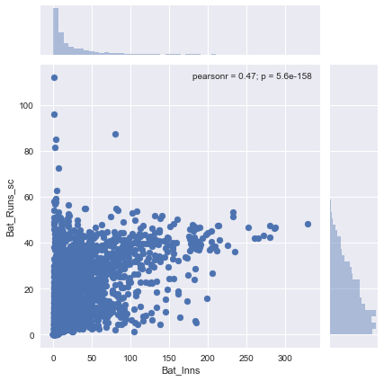
Clearly this is a far better representation of batting capabilities of a player. You can see there is less dependency on the number of innings played. It is not hard to imagine how this scaling affects our final prediction. The impact is obvious when we plot batting runs and bowling wickets (likely to be the most important features) in a KDE plot. Here is the KDE plot before scaling:
sns.jointplot(x="Bowl_Wkts", y="Bat_Runs", data=df,kind='kde')
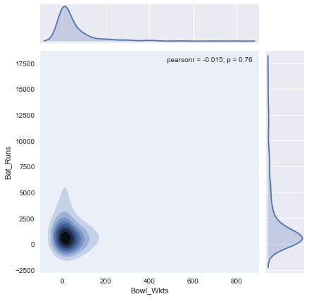
There is no clear clustering indicating that our classification is not going to be effective. In comparison, if we generate the same chart for scaled values, there is a clear grouping.
sns.jointplot(x="Bowl_Wkts_sc", y="Bat_Runs_sc", data=df,kind='kde')
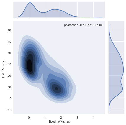
This much more promising. Remember, your model will only perform as well as the data you feed in. If the input data is already confused, there is very little a mathematical model can do. Now that we have almost all that we need we will extract those records that have playing role information and use it for our training & testing. To avoid outliers corrupting our model, we will also exclude players who played less than 5 matches.
# remove players who played less than 5 matches
df = data[data['Bio_Playing_role'].notnull() & (data['Bat_Mat'] > 5)]
Data Transformation
Next let us look at our target feature which is playing role. We need to understand the values it can assume. Let us look at the unique values for the player features.
# Check the unique playing roles to identify mapping function
data['Bio_Playing_role'].unique()
array([nan, 'Top-order batsman', 'Bowler', 'Middle-order batsman',
       'Wicketkeeper batsman', 'Allrounder', 'Batsman', 'Opening batsman',
       'Wicketkeeper', 'Bowling allrounder', 'Batting allrounder'], dtype=object)
The playing role definition is too granular. We want fewer variety of roles so that each role gets sufficient sample data points to train the model. Also the role tagging done by Cricinfo is not consistent. For e.g., not all opening batsmen have been tagged with the opening batsman role. So we define a mapping function to group playing roles in to 4 different categories ['Batsman','Bowler','Wicketkeeper','Allrounder']
def get_role(role):
    if  pd.notnull(role):
        if 'keeper' in role:
            return "Wicketkeeper"
        elif 'rounder' in role:
            return "Allrounder"
        elif 'atsman' in role:
            return "Batsman"
        elif 'owler' in role:
            return "Bowler"
        else:
            return ""
    else:
        return ""

data['role'] = data['Bio_Playing_role'].apply(get_role)
Note that this feature is a categorical data. It is different from a numerical data such as height or weight. When we want to use Deep Neural Networks we need to represent the target features as numerical data. We will assign one column for each playing role and set its value to one when that playing role fits the player well. Then the function of our model will be to assign a value close to 1 for one of these columns and a value close to 0 for the rest.
It is called One-Hot encoding. Turns out this is a frequent task, so pandas has a handy inbuilt function to perform this.
# y is categorical feature
y = df['role']

# Convert categorical data into numerical columns
y_cat = pd.get_dummies(y)

# X is the input features. We need to covert it from pandas dataframe to numpy array to feed in to our models
X = df[features].as_matrix()
Let us see the new y_cat dataframe
y_cat.head()
| Allrounder | Batsman | Bowler | Wicketkeeper | |
|---|---|---|---|---|
| 19 | 0 | 1 | 0 | 0 |
| 20 | 0 | 0 | 1 | 0 |
| 22 | 0 | 0 | 0 | 1 |
| 25 | 1 | 0 | 0 | 0 |
| 28 | 0 | 1 | 0 | 0 |
One might be tempted to assign unique numbers for each category ( say 1: Batsman, 2: Bowler etc.,) but that will not work. There is no quantitative relation between categories. Assigning raw numbers implies that there is a numerical progression to the categories. Sometimes it can work for contiguous data such as day of the month, but even then one has to be aware of the bounds and circularity of the target variables.
Scaling data
Some fields vary over a larger range compared to the rest. Remember we did a preliminary scaling by dividing these values with the number of innings. But that is not sufficient since it only made sure that one feature (’no. of innings’) did not overtly influence another feature (‘runs scored’). But each features themselves lie between different extremities. For e.g, Bowling Wickets Scaled only ranges from 0 to 5 whereas Batting Runs Scaled ranges from 0 to 50. Most machine learning models works the best when the features are vary within the same range. If we let these datapoints influence our calculation without modification, wickets taken will have negligible influence.
So we perform another round of scaling for all input data points. We will use the MinMax Scaler from Scikit library. This will scale the values such that largest value becomes one and smallest value becomes zero.
from sklearn.preprocessing import MinMaxScaler
mms = MinMaxScaler(feature_range=(0,1)).fit(X)

# X_mms will our new input array with all values scaled to be between 0 and 1
X_mms = mms.transform(X)
Training the model
Deep Neural Network
First we will try to run a Deep Neural Network model on this data. Here are the necessary modules to import.
from keras.models import Sequential
from keras.layers import Dense
from keras.optimizers import SGD, Adam, Adadelta, RMSprop
from keras.wrappers.scikit_learn import KerasClassifier
import keras.backend as K
Create the Keras Sequential model. I am using a DNN with 1 hidden layer and 1 output layer. The hidden layer has 15 nodes. The number of nodes in the output layer should as the number of categories. So we will go with 4.
def create_baseline():
    # create model
    model = Sequential()
    model.add(Dense(15, input_dim=25, kernel_initializer='he_normal', activation='relu'))
    model.add(Dense(4, kernel_initializer='he_normal', activation='softmax'))
    # Compile model
    model.compile(loss='categorical_crossentropy', optimizer='adam', metrics=['accuracy'])
    return model
The softmax is a popular activation function for classification problems. In simple words, an activation function is a simple function that decides whether to output TRUE or FALSE for each category. This softmax function receives an array of values from the previous layer and returns a new array which adds up to 1. The category with the largest value is deemed likely match for our data.
Softmaxhighlights only the likeliest category for a data. Here for simplicity sake, we assume that our categories are mutually exclusive, i.e, a player can only belong to one category at a time. There are other data types where a single entry can belong to more than one category at a time. We may need to use different activation function for that. Again, know your data before deciding on activation function.
The loss function is categorical_crossentropy. A Loss Function can be thought of as a course correction function which measures the perceived error as our model navigates to ideal set of weights over multiple iterations. Categorical Cross-Entropy loss function penalizes weights that are sure to be wrong. It is a common loss function used for classification problems.
These are the important attributes that closely follows our problem definition. Most of the other parameters can be fiddled with.
Next we will use Keras to train the model. The result is a Keras Classifier function whose weights are trained on our data. We can use this function to predict values for inputs which we haven’t seen so far.
# evaluate model with standardized dataset
estimator = KerasClassifier(build_fn=create_baseline, nb_epoch=100, batch_size=5, verbose=0)
We cannot use all of the data to train our model. The model will closely follow our existing model. It won’t be useful to predict any values we haven’t seen so far. This is called overfitting.
To avoid this, we will split the data into train and test datasets. We will use the former to train the model and compute the scores based on the testing against test data for each iteration of cross-validation. Scikit’s provides a helper function called cross_val_score to assist in this. StratifiedKFold is the genertor strategy we will use for selecting this train/test datasets. It splits the data into K folds (set to 10 in our case), trains it on K-1 datasets and tests it against the left out dataset, while preserving the class distribution of the data.
# set the random state to a fixed number for reproducing the results
kfold = StratifiedKFold(n_splits=10, shuffle=True,random_state=42)
results = cross_val_score(estimator, X_mms, y.values, cv=kfold)
print("Results: %.2f%% (%.2f%%)" % (results.mean()*100, results.std()*100))
I got a result of 82.2% accuracy. Not bad for the first attempt, particularly since we employed gross simplifications and trained the model with only with around 450 records. The results that you get may be slightly different since we shuffle the data before generating folds.
Random Forest Classifier
This time let us try to model the data using Random Forest classifier. Random Forest Classifier is a much simpler method than neural networks. It relies on building multiple decision trees and assembling the results of these decision trees.
from sklearn.ensemble import RandomForestClassifier

# Instantiate model with 1000 decision trees
rf_estimator = RandomForestClassifier(n_estimators = 1000, random_state = 42)

rf_results = cross_val_score(rf_estimator, X_mms, y.values, cv=kfold)
print("Results: %.2f%% (%.2f%%)" % (rf_results.mean()*100, rf_results.std()*100))
You will notice that Random Forest Classifier has performed significantly better than the DNN classifier. I got 87.28% accuracy, which is amazing since Random Forest is several times faster and less resource intensive than the DNN classifier. And I didn’t even have to run it on top of tensorflow and make use of GPU. Decision trees are quite effective at classification tasks but they tend to overfit.
Reviewing the results
Since our Random Forest model has performed significantly better, we will use that model to predict the unseen roles of players.
# Fit the estimator on available data
rf_estimator.fit(X_mms, y.values)

# np array to hold all of the input data
P = data[features].as_matrix()

# An ugly hack to drop infinity values introduced as part of some of the pre-processing tasks
P[P > 1e308] = 0

# Min Max Scaling
P_mms = min_max_scaler.fit_transform(P)

# Prediction based on the Random forest model
data['predicted_role_rf'] = rf_estimator.predict(P_mms)
Confusion Matrix
A score alone is not a good indicator that our model has performed well. We need to review its performance by plotting Confusion Matrix. It is a simple matrix plot based on known test data with predicted values plotted against the true value. The diagonal entries represent correct prediction, rest represents confused values. Let us plot Confusion Matrix for our data.
from sklearn.metrics import confusion_matrix
mat = confusion_matrix(data[(data['role']!='')]['role'],
                       data[(data['role']!='')]['predicted_role_rf'],
                       labels = ['Batsman','Bowler','Allrounder','Wicketkeeper'])
sns.heatmap(mat.T, square=True, annot=True, fmt='d', cbar=False)
plt.xlabel('true label')
plt.ylabel('predicted label')
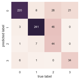
We can see that the model is quite effective in matching the pure roles such as Batsman or Bowler. When it comes to mixed roles such as Allrounder or Wicketkeeper, it fares not that well. Part of the problem lies in our assumption that the roles are mutually exclusive i.e, a player cannot be both Batsman and Bowler at the same time. So we identify only around 37% of the all rounders successfully. Later we will see that there are other reasons why the predicted role doesn’t match the role marked in cricinfo.
Reviewing the results
Let us see the cases where our predictions differed from the roles defined in cricinfo:
data[(data['role'] != data['predicted_role_rf']) & (data['role'] != '') & (data['Bat_Mat'] > 5 )][['Bio_Full_name','predicted_role_rf', 'role', 'Bio_Playing_role']]
I have extracted the differences for popular players of recent times. Subjectively speaking our model hasn’t performed too bad. There seems to be some merit to the classification offered by the model compared to the playing role assigned in cricinfo bio page.
| Bio_Full_name | predicted_role_rf | role | Bio_Playing_role | |
|---|---|---|---|---|
| 38 | Stephen Norman John O’Keefe | Bowler | Allrounder | Allrounder |
| 44 | Glenn James Maxwell | Batsman | Allrounder | Batting allrounder |
| 88 | Andrew Symonds | Batsman | Allrounder | Allrounder |
| 227 | Shai Diego Hope | Batsman | Wicketkeeper | Wicketkeeper batsman |
| 281 | Brendon Barrie McCullum | Batsman | Wicketkeeper | Wicketkeeper batsman |
| 970 | Angelo Davis Mathews | Batsman | Allrounder | Allrounder |
| 1437 | Abraham Benjamin de Villiers | Batsman | Wicketkeeper | Wicketkeeper batsman |
In most cases, Cricinfo’s playing role is also based on the ODI and T20 formats. Some of the players like ABD Villiers and Brendon McCullum have donned multiple roles but given up gloves for the games longest format. So we can’t really fault the model here for identifying them as batsman. Then there are other cases of a player being regarded as All rounder based on the role they play in shorter formats.
Next to the most interesting part- let us see how our model behaves for the data it hasn’t seen i.e., the classification of those players whose playing role is missing in their bio page. For ease of identification, I have filtered only those players who have played 100 matches or more.
data[(data['role'] != data['predicted_role_rf']) & (data['role'] == '') & (data['Bat_Mat'] > 100 )][['Bio_Full_name','predicted_role_rf', 'role', 'Bio_Playing_role']]
| Bio_Full_name | predicted_role_rf | role | Bio_Playing_role | |
|---|---|---|---|---|
| 134 | Mark Edward Waugh | Batsman | NaN | |
| 137 | Mark Anthony Taylor | Batsman | NaN | |
| 139 | Ian Andrew Healy | Wicketkeeper | NaN | |
| 599 | Sourav Chandidas Ganguly | Batsman | NaN | |
| 743 | Anil Kumble | Bowler | NaN | |
| 925 | Brian Charles Lara | Batsman | NaN | |
| 929 | Carl Llewellyn Hooper | Batsman | NaN | |
| 937 | Courtney Andrew Walsh | Bowler | NaN | |
| 957 | Desmond Leo Haynes | Batsman | NaN | |
| 1072 | Kapildev Ramlal Nikhanj | Bowler | NaN | |
| 1074 | Dilip Balwant Vengsarkar | Batsman | NaN | |
| 1088 | Sunil Manohar Gavaskar | Batsman | NaN | |
| 1257 | Cuthbert Gordon Greenidge | Batsman | NaN | |
| 1258 | Isaac Vivian Alexander Richards | Batsman | NaN | |
| 1284 | Clive Hubert Lloyd | Batsman | NaN | |
| 1326 | Warnakulasuriya Patabendige Ushantha Joseph Chaminda Vaas | Bowler | NaN | |
| 1463 | Makhaya Ntini | Bowler | NaN | |
| 1474 | Gary Kirsten | Batsman | NaN | |
| 1676 | Alec James Stewart | Batsman | NaN | |
| 2020 | Inzamam-ul-Haq | Batsman | NaN | |
| 2168 | Graham Alan Gooch | Batsman | NaN | |
| 2205 | Wasim Akram | Bowler | NaN | |
| 2216 | Saleem Malik | Batsman | NaN | |
| 2320 | Geoffrey Boycott | Batsman | NaN | |
| 2366 | Michael Colin Cowdrey | Batsman | NaN | |
| 2381 | Mohammad Javed Miandad Khan | Batsman | NaN |
Even a cursory look can tell us that our model worked splendidly. It is surprising how many prominent player bio pages has their playing role information missing. Well, it looks like even a simple ML model can fix that gap.
Let us see how the two most critical features (Bat_Runs_sc and Bowl_Wkts_sc) affects our predicted role.
sns.set_palette("bright")
sns.lmplot('Bowl_Wkts_sc','Bat_Runs_sc',data[data['Bat_Mat'] > 5 ],
           hue='predicted_role_rf', fit_reg=False, size=10)
    plt.plot([0,7.0],[100,0])
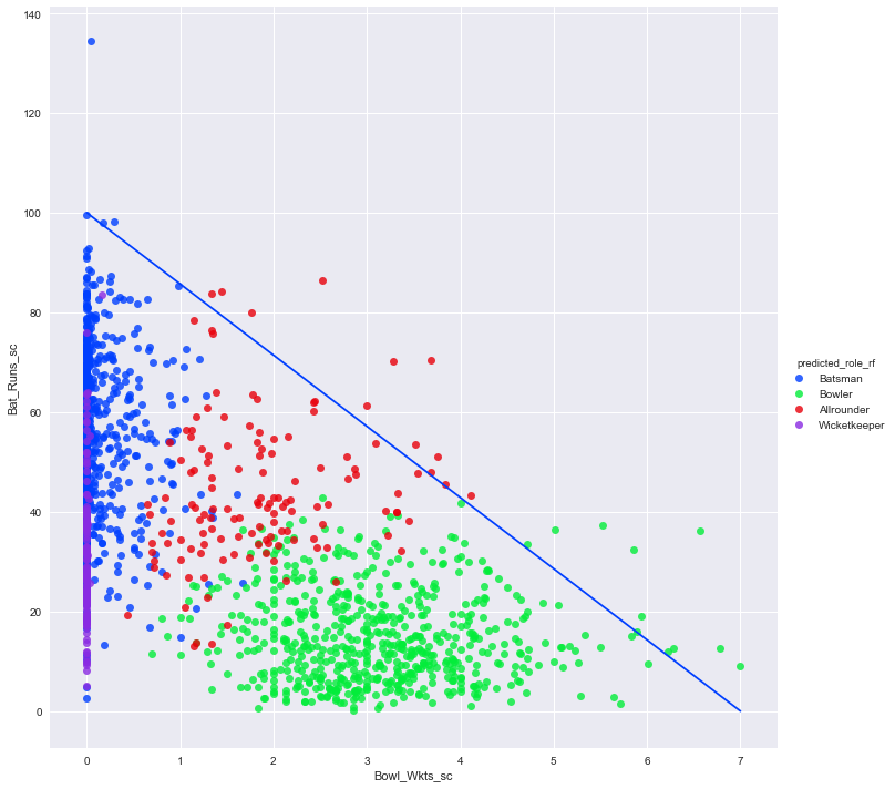
I have plotted a diagonal line, below which most of the points are clustered. It represents a kind of pareto-frontier which only exceptional players can breach. Note that there is no statistical basis for my choice of x and y intercepts, I just based it on visual inspection. Let us see the list of players who reside above this threshold.
data[data['Bat_Mat'] > 5].query('Bowl_Wkts_sc*100 + Bat_Runs_sc*7 > 700 ')[['Bio_Full_name','Bat_Mat','predicted_role_rf','Bowl_Wkts_sc','Bat_Runs_sc']]
| Bio_Full_name | Bat_Mat | predicted_role_rf | Bowl_Wkts_sc | Bat_Runs_sc | |
|---|---|---|---|---|---|
| 62 | Steven Peter Devereux Smith | 59 | Batsman | 0.288136 | 98.237288 |
| 377 | Ravindrasinh Anirudhsinh Jadeja | 35 | Bowler | 4.714286 | 33.600000 |
| 380 | Ravichandran Ashwin | 55 | Bowler | 5.527273 | 37.363636 |
| 456 | Christopher Lance Cairns | 62 | Allrounder | 3.516129 | 53.548387 |
| 526 | Shakib Al Hasan | 51 | Allrounder | 3.686275 | 70.470588 |
| 720 | Sikandar Raza Butt | 9 | Allrounder | 1.444444 | 84.111111 |
| 832 | Donald George Bradman | 52 | Batsman | 0.038462 | 134.538462 |
| 1133 | Herbert Vivian Hordern | 7 | Bowler | 6.571429 | 36.285714 |
| 1177 | Richard John Hadlee | 86 | Bowler | 5.011628 | 36.325581 |
| 1240 | Yasir Shah | 28 | Bowler | 5.892857 | 15.892857 |
| 1468 | Jacques Henry Kallis | 166 | Allrounder | 1.759036 | 80.054217 |
| 1548 | Charles Thomas Biass Turner | 17 | Bowler | 5.941176 | 19.000000 |
| 1748 | Garfield St Aubrun Sobers | 93 | Allrounder | 2.526882 | 86.365591 |
| 1825 | Michael John Procter | 7 | Bowler | 5.857143 | 32.285714 |
| 1838 | Robert Graeme Pollock | 23 | Batsman | 0.173913 | 98.086957 |
| 1849 | Edgar John Barlow | 30 | Allrounder | 1.333333 | 83.866667 |
| 1860 | Trevor Leslie Goddard | 41 | Allrounder | 3.000000 | 61.365854 |
| 2157 | Ian Terence Botham | 102 | Allrounder | 3.754902 | 50.980392 |
| 2285 | Mulvantrai Himmatlal Mankad | 44 | Allrounder | 3.681818 | 47.931818 |
| 2386 | Imran Khan Niazi | 88 | Allrounder | 4.113636 | 43.261364 |
| 2522 | George Aubrey Faulkner | 25 | Allrounder | 3.280000 | 70.160000 |
| 2741 | George Joseph Thompson | 6 | Allrounder | 3.833333 | 45.500000 |
| 2769 | Sydney Francis Barnes | 27 | Bowler | 7.000000 | 8.962963 |
| 2809 | Thomas Richardson | 14 | Bowler | 6.285714 | 12.642857 |
| 2821 | John James Ferris | 9 | Bowler | 6.777778 | 12.666667 |
| 2845 | George Alfred Lohmann | 18 | Bowler | 6.222222 | 11.833333 |
The list is dominated by exceptional all-rounders. Among specialists, bowlers fare better. Perhaps it is my fault that I set the bar for greatness too high. The Bat_Runs_sc of Bradman is so far ahead of the rest, that it one tends to choose a higher value for y-intercept.
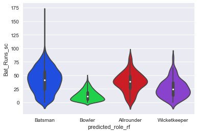
Finally let us plot Bat_Runs_sc against predicted playing role using a violin plot. This will shows distribution of runs scored across the multiple categories of playing role. We can see that for batsmen, the bulk of the violin plot is top heavy whereas for the bowlers it is bottom heavy.
sns.violinplot(x='predicted_role_rf',
               y='Bat_Runs_sc',
               data=data,
               scale='width')
Conclusion
If you review the length of the posts, less than 20% is allocated to running the actual machine learning code. That closely reflects the time spent on this project as well. Bulk of the time is spent in collecting and curating the data. Also the results from RandomForest Classifier is revealing. Right tool for the right job is often more effective than a generic tool which is universally useful.
Machine Learning and Data science is a vast subject. Despite the length of this post, I have barely touched the surface of this domain. Apart from the knowledge of tools and procedures, one needs to have a good understanding of the data and be conscious of the inherent biases in the numerical models.
Finally, scikit-learn is an excellent resource for learning and practising Machine learning. It has excellent documentation and helper functions for many of the common tasks. I found Python Data Science Handbook to be another great freely available resource.